R package Tutorial

Introduction

The R package tutorial can ve directly viewed in the R console with the command browseVignettes("cliqueMS") assuming you have R package installed.

Untargeted metabolomics goal is to quantify as metabolites as possible from a sample. We can use liquid chromatography coupled to mass spectrometry (LC/MS) for this purpose. It is a great challenge to transform LC/MS data into a profile of annotated metabolites that provides us meaningful biological information. A very important limitation to the annotation of metabolomic experiments is that the number of m/z processed signals, called features, is much bigger than the putative number of metabolites in a sample. The sources that produce multiple features from a single metabolite are multiple and variable. Natural isotopes as carbon isotopes produce isotope features. Ionization of metabolites produce the so called adducts of the metabolite, which are detected as different features depending on the ion adduct involved ([M+Na]+, [M+H]+, etc..). Apart from adduct features, ionization also produces metabolite fragmentation and other reactions as dimerizations, trimerizations, all of them being detected as multiple features. Being the reduction of multiple features to single metabolites a crucial step for the correct annotation of LC/MS experiments, we will show how to use cliqueMS to do so.

cliqueMS annotates samples one by one. Annotation can be summarised in these three steps:

1. Divide features into clique groups.
2. Annotate isotopes.
3. Annotate adducts and fragments.

Annotation steps are stored in an anClique S3 object. This object can be created from a XCMSnExp or a xcmsSet object with processed m/z data from xcms package. First m/z raw data is processed:

Then we can create an anClique object:

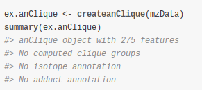
Here we see an anClique object before any annotation step. Features have not been grouped, isotopes and adducts are not annotated. Now let’s see the three steps in detail.

Metabolites produce multiple features and very often they do not separate completely in the chromatography, so we observe coelution. This increases the difficulty of the annotation because many features coming from different metabolites might appear very close in the chromatogram. Before trying to annotate isotopes, adducts and fragments we want to make groups of features. Ideally, each group should include all the features produced by a single metabolite.

cliqueMS uses a similarity network to find groups of features. Each feature is a node, and edges are weighted according to the cosine similarity between features:

Values from cosine similarity are useful to discriminate pairs of features that come from the same metabolite from pairs of features that come from different metabolites [1]. We compute the cosine similarity using the profile mode of the data, having each feature a m/z value and vector intensities. All features are discretized into a vector of equal bins κ. Each vector position relative to retention time τ_κ contains the intensity of the feature ι_κ at that moment of the chromatography. Features with no coelution at all have a cosine similarity = 0. Edges with weight = 0 are not included in the network, nor nodes without any edge.

Once we have the network, it is time to divide the features into groups. cliqueMS assumes that the similarity between all features that come from the same metabolite must be c_ij>0. Additionally, similarity values between features of the same metabolite should be generally higher than between features of different metabolites. With this information, cliqueMS uses a probabilistic model to find the feature groups. This model find cliques, fully connected components so for all nodes c_ij>0. The similarity inside this cliques should be higher than the similarity between features outside the clique. cliqueMS estimates the log-likelihood for a particular assignment of features into different clique groups. For details in the probabilistic model and the log-likelihood maximisation see [1]. The log-likelihood maximisation procedure can be summarised in the following way:

1. cliqueMS starts with each node as a different clique group.
2. Alternate between merge cliques and move nodes from cliques if the new assignment has a bigger log-likelihood.
3. When log-likelihood cannot be increased in 2, try to move each node from its clique to another, (“Kernighan-Lin”).
4. Final group assignment for all features.

Now let’s see how to find this groups with getCliques.

With the function getCliques we assign clique groups to our features. This function creates the network of similarity and then computes the clique groups. As input data it uses a xcmsSet or XCMSnExp object. getCliques outputs an anClique S3 object, which will be used to store all annotation steps.

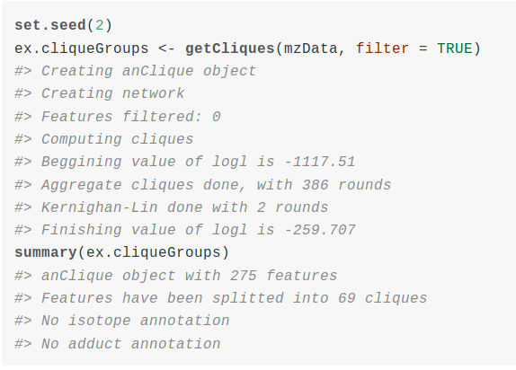
As we see from the printed messages, the function getCliques first creates a network, and then it filters features if parameter filter = TRUE . As m/z signal processing algorithms may produce two artefact features from a single one, it is recommended to set filter = TRUE to drop repeated features. This filter only drops features with similarity > 0.99, and equal values of m/z, retention time and maximum intensity, defined by the relative error parameters mzerror , rtdiff and intdiff . From the output of the function we see the computed log-likelihood at the beginning, when each feature is in a different clique and the computed log-likelihood at the end of the process. If we now look at the summary of the resulting anClique object, we see that the features have been grouped into 69 clique groups. Now we can annotate isotopes.

cliqueMS annotates isotopes within each clique group. cliqueMS searches pairs of features than can be carbon isotopes based in these two rules:

1. The monoisotopic feature must be more intense than the isotopic feature.
2. The mass difference between the features must be the difference of a carbon isotope ± an error.

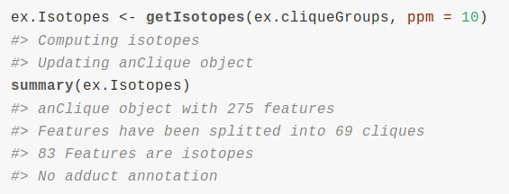
Isotopes are annotated with the function getIsotopes . This function finds pairs of features that fulfil the conditions of an isotope. Then it creates the isotope annotation after removing incoherences like two monoisotopic masses for one isotope, two second isotopes for one first isotope, etc… In all this cases the removed pair is the one with smaller similarity. The use of the function is pretty straightforward:

Parameter ppm is important because it defines in ppm units the range of the accepted relative error. Once isotopes are annotated we can annotate adducts and fragments.

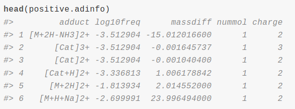
The last step of cliqueMS is to annotate adducts. Each feature has a m/z value that is the neutral mass of the metabolite plus the mass of the ion adduct (or fragmentation ion adduct). The neutral mass is an unknown value, but the ion adduct mass is to some degree known as many ion adducts are known. The list of possible adducts should be given as input to cliqueMS by the user or either use one of the default adduct lists. Here is how it looks the positive default list:

Which contains the name of the adduct, the log10 frequency of that adduct, the mass of the adduct, the number of molecules involved and the charge (see [1] for details in how default lists were made). With the adduct list we can obtain neutral masses.

Scoring neutral masses

cliqueMS searches in each clique for groups of two or more features compatible with a neutral mass and two or more adducts in the adduct list. Neutral masses with only one adduct are not included in the scoring. Once we have all possible neutral masses and their corresponding adducts, the algorithm tries combinations of different adducts and neutral masses to find the most plausible annotation. All combinations are scored and the top five annotations are returned. The scoring is based on the following criteria:

1. The log-frequency of the adduct
2. Minimum number of empty features
3. Minimum number of neutral masses

The computed score (which is a logarithmic score) is the sum of the adducts log-frequencies plus the number of empty features (which has a log-frequency smaller than the least frequent adduct) and the number of neutral masses. Within a clique group, it may happen than the annotation of some features is independent from the annotation of some other features, as there is not a single neutral mass with adducts in both groups of features. In those cases, the clique group is splitted in non overlapping groups, called annotation groups. This is common in big cliques. The reported scores refer to annotation groups. The score is useful to see how probable is the first annotation compared to second annotation, third annotation, etc… within an annotation group, but it is not intended to compare annotations between different annotation groups because the score will be smaller when the number of features in the group is bigger.To compare scores from different groups, the option normalizeScore should be set to TRUE . The normalized score value is 100 when the score is similar to the theoretical maximum score (all the features annotated with the most frequent adducts and the minimum number of neutral masses) and goes until 0, which is the extreme case that all features of the group are not annotated. To find annotation cliqueMS uses the function getAnnotation .

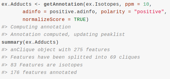
Here is an example of annotating adducts with getAnnotation :

As we see from the summary output, 178 of 275 features have annotation. Function getAnnotation requires as input an adduct list, the parameter adinfo . Users can use the default adduct list positive.adinfo for positive charged adducts and negative.adinfo for negative charged adducts. polarity must be set, either to positive or negative . Lots of neutral masses are found when the clique groups have many features. In those cases, scoring all annotations could take much time as there are many possible combinations. To prevent this, neutral masses that likely will be in the final top annotations are selected and annotation is computed quickly. The selected masses have the highest frequency adducts and the largest number of adducts. For each clique group, all neutral masses are ordered depending on their score. A number of top scoring masses controlled by topmasstotal parameter are selected. Additionally and for every feature, the ordered list of scored neutral masses is subsetted to only the neutral masses with adducts in that feature. Then a number of top scoring masses set by topmassf parameter are selected in each sublist, and added to the set of selected masses. After the mass selection, and in cases of big cliques (size of a “big” clique is defined by parameter sizeanG ), annotation groups are splitted again in new non overlapping groups just taking into account the set of selected neutral masses.

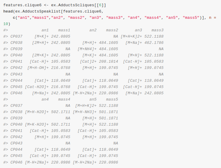
getCliques stores the annotation in the peaklist of the anClique object. Here we can see an overview of some annotated features in our sample:

Now we have obtained the neutral mass and the adduct annotation for our features. We could use the neutral mass together with the retention time and MS/MS data to annotate more confidently some of these metabolites. We also know how many features in the dataset are isotopes. Finally, we have achieved a reduction in the complexity of our the dataset, from many features to a signficant smaller number annotated neutral masses that have different adducts and isotopes.